Efficiency & Limitations

Learning Objectives

After reading this chapter, you will be able to:

• Design experiments to measure time and space overhead for private algorithms

• Consider tradeoffs between space and time efficiency

• Consider techniques for optimization

• Describe the efficiency bottlenecks in differentially private algorithms

• Describe limitations of differential privacy

Time Efficiency of Differential Privacy

In a situation where the application of differential privacy is implemented as a direct loop over sensitive entities, there is a significant time cost incurred from the added burden of random number generation.

We can contrast the runtime performance of two versions of a counting query - one with differential privacy, and one without it.

import itertools
import operator
import time

def time_count(k):   
    l = [1] * k
    start = time.perf_counter()
    _ = list(itertools.accumulate(l, func=operator.add))
    stop = time.perf_counter()
    return stop - start 

def time_priv_count(k):  
    l = [1] * k
    start = time.perf_counter()
    _ = list(itertools.accumulate(l, func=lambda x, y: x + laplace_mech(y,1,0.1), initial=0))
    stop = time.perf_counter()
    return stop - start 

x_axis = [k for k in range(100_000,1_000_000,100_000)]
plt.xlabel('Size (N)')
plt.ylabel('Time (Seconds)')
plt.plot(x_axis, [time_count(k) for k in range(100_000,1_000_000,100_000)], label='Regular Count')
plt.plot(x_axis, [time_priv_count(k) for k in range(100_000,1_000_000,100_000)], label='Private Count')
plt.legend();

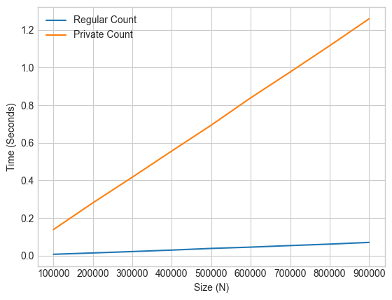
With the time spent counting on the y-axis, and the list lize on the x-axis, we can see that the time complexity of differential privacy for this particular operation is essentially linear in the size of the input.

The good news is that the above implementation of differentially private count is rather naive, and we can do much better using optimization techniques such as vectorization!

For example, when implementing differential privacy for the machine learning operations in a previous chapter, we make use of NumPy functions which are heavily optimized for vector-based operations. In this particular scenario, leveraging this strategy, we manage to incur negligible time cost for the use of differential privacy.

delta = 1e-5

def time_gd(k):   
    start = time.perf_counter()
    gradient_descent(k)
    stop = time.perf_counter()
    return stop - start 

def time_priv_gd(k):   
    start = time.perf_counter()
    noisy_gradient_descent(k, 0.1, delta)
    stop = time.perf_counter()
    return stop - start 

x_axis = [k for k in range(10,100,25)]
plt.xlabel('Size (N)')
plt.ylabel('Time (Seconds)')
plt.plot(x_axis, [time_gd(k) for k in range(10,100,25)], label='Regular GD')
plt.plot(x_axis, [time_priv_gd(k) for k in range(10,100,25)], label='Private GD')
plt.legend();

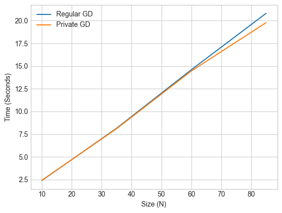
The graph plots generally overlap or are close in most simulations of this experiment, indicating low (constant) time inefficiency overhead incurred from utilizing private gradient descent.

Increased Iterations in Model Training Under Differential Privacy

When noise is introduced into model training to ensure differential privacy, it often results in a need for more iterations—such as additional training steps or epochs—before the model converges to an acceptable level of performance.

This increase in training time is primarily due to the way noise disrupts the learning process. Differential privacy mechanisms like DP-SGD (Differentially Private Stochastic Gradient Descent) work by adding noise to the gradients during optimization. These gradients are computed from small batches of data, and the added noise is designed to obscure the influence of any single data point. While this is effective for privacy protection, it also has the side effect of making the gradients noisier and less informative. The optimizer receives a weaker signal about the true direction to move in the loss landscape, which can slow down learning.

To manage the instability introduced by noise, practitioners often use smaller learning rates. Smaller step sizes help avoid erratic behavior but also result in slower convergence. The combination of less reliable gradients and more cautious updates means that it usually takes longer for the model to reach a useful solution. In many cases, this means training for more epochs, evaluating more checkpoints, and possibly using early stopping with looser tolerances.

In practice, this means that training models under differential privacy not only demands more iterations but also more careful tuning of hyperparameters like the learning rate, batch size, clipping norm, and noise multiplier. For example, previously in this book, we compare training logistic regression models with and without differential privacy and observe that the model trained with DP converges more slowly and reaches a lower maximum accuracy. This is consistent with what is observed in the literature: differential privacy makes learning harder, but with the right strategies and sufficient computation, useful models can still be trained.

Space Cost of Differential Privacy

We can also analyze the space utilization of differential privacy mechanisms. Python3 (3.4) introduces a debug tool capable of tracing memory blocks allocated for use during evaluation. We may perform our analysis of space overhead by comparing the peak size of memory blocks used during private versus non-private computation.

Using this strategy, we can analyze the space overhead of the private count operation as follows:

import itertools
import operator
import tracemalloc

def space_count(k):   
    l = [1] * k
    itertools.accumulate(l, func=operator.add)
    _, peak = tracemalloc.get_traced_memory()
    tracemalloc.reset_peak()
    return peak/1000 

def space_priv_count(k):  
    l = [1] * k
    itertools.accumulate(l, func=lambda x, y: x + laplace_mech(y,1,0.1), initial=0)
    _, peak = tracemalloc.get_traced_memory()
    tracemalloc.reset_peak()
    return peak/1000

tracemalloc.start()
x_axis = [k for k in range(100_000,1_000_000,100_000)]
plt.xlabel('Size (N)')
plt.ylabel('Memory Blocks')
plt.plot(x_axis, [space_count(k) for k in range(100_000,1_000_000,100_000)], label='Regular Count')
plt.plot(x_axis, [space_priv_count(k) for k in range(100_000,1_000_000,100_000)], label='Private Count')
tracemalloc.stop()
plt.legend();

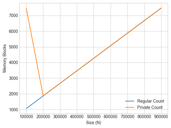
We display every thousand memory blocks on the y-axis, against the list size on the x-axis.

In this case, the memory complexity of differential privacy is generally constant.

We also observe a spike in the initial space cost for private count, which we can attribute to memory allocation for setup of the random number generator resources such as the entropy pool and PRNG (pseudo-random number generator).

We can repeat this experiment to contrast private and non-private machine learning:

def space_gd(k):   
    gradient_descent(k)
    _, peak = tracemalloc.get_traced_memory()
    tracemalloc.reset_peak()
    return peak/1_000_000 

def space_priv_gd(k):   
    noisy_gradient_descent(k, 0.1, delta)
    _, peak = tracemalloc.get_traced_memory()
    tracemalloc.reset_peak()
    return peak/1_000_000

tracemalloc.start()
x_axis = [k for k in range(5,10,2)]
plt.xlabel('Size (N)')
plt.ylabel('Memory Blocks')
plt.plot(x_axis, [space_gd(k) for k in range(5,10,2)], label='Regular GD')
plt.plot(x_axis, [space_priv_gd(k) for k in range(5,10,2)], label='Private GD')
tracemalloc.stop()
plt.legend();

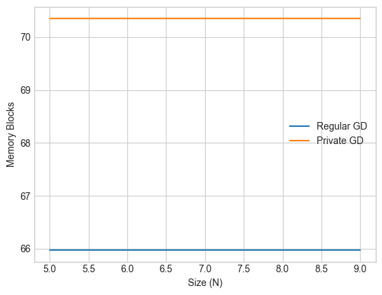
In this case, since we are performing gradient descent, the memory allocation is generally much larger - as expected - so we graph against every millionth allocated memory block.

We also observe generally constant space overhead during private gradient descent. However the space overhead is much larger here since we leverage extra space for vectorization and concurrency to improve time efficiency.

Note

Ghost Clipping in Differential Privacy

Ghost clipping is a technique introduced to improve both time and space efficiency when training differentially private models—especially in private deep learning with private Large Language Models (LLMs).

Rather than instantiating and modifying per-sample gradients directly during training, Ghost Clipping works directly from per-sample activation gradients and per-sample activations, avoiding the need for gradient instantiation.

This technique is utilized in tools like Opacus by Meta and TensorFlow Privacy by Google.

You can read more about ghost clipping here as described in the academic paper and here in the Pytorch blog.

Limitations of Random Number Generation

In conclusion, while some bottlenecks may exist, there are techniques we can use to keep both the space and time cost of differential privacy generally low (constant) throughout the lifetime of program evaluation.

Why do any bottlenecks exist, and why are they particular to differential privacy? In order to preserve the guarantee of differential privacy, we require high-quality entropy. This is a limited resource because it generally relies on some external source of non-deterministic environmental input. Examples of non-determinintic entropy sources can include disk/network IO, keyboard presses, and mouse movement.

Usually this entropy is stored in some special buffer or file to be retrieved and used later on.

with open("/dev/random", 'rb') as file:
    print(file.read(8))

b'\x11\x83JI\x93x\xff,'

Alternatively, we could use:

import os
os.urandom(32)

b'L\x0b\xb43\xab\xc3\x03\x9c\x016z\x92`\xd4\xa7\x90F0%\xcb\xc6p\xe4F\r\x1f\xdf\x00\xcc\xab\x8f\xe2'

Or:

import secrets 
secrets.token_bytes(32)

b'\xcc\xa1A\xce@aqU~c\x10B\xf5\x9e\xb8!\xa0#5MTn\xf69r\xe6\x97\x96\x05\x8e\x1c\x87'

In general, in different programming languages and operating systems, there are several options for random number and seed generation, with varying applicability for use cases such as: modeling, simulation, or production of cryptographically strong random bytes suitable for managing sensitive user data at scale.

Real Numbers and Random Noise

Differential privacy relies on randomized mechanisms that add noise drawn from continuous distributions — most commonly, the Laplace or Gaussian distributions. These distributions are defined over the real numbers, but real numbers cannot be represented exactly on a computer. Instead, we use floating-point approximations, which can introduce subtle but significant issues.

In practice, when we generate random noise (e.g., using np.random.laplace() in NumPy), we’re relying on finite-precision arithmetic. While this generally works well enough for most use cases, it opens the door to deterministic behavior at the tails of the distribution, or small variations that can be exploited in attacks.

In a landmark paper, Ilya Mironov showed that the naive implementation of the Laplace mechanism using floating-point arithmetic can leak private information through subtle artifacts in the generated noise values — particularly due to non-uniform spacing of representable floats. These artifacts can produce discontinuities or patterns in the output distribution that a clever adversary can detect and exploit [14].

To mitigate these risks, several strategies have been proposed:

• Carefully engineered sampling algorithms, such as Mironov’s Snapping Mechanism, which aligns output to a uniform floating-point grid while preserving differential privacy.

• Using discrete noise distributions (e.g., geometric or discrete Laplace) as approximations that are easier to reason about in finite-precision settings.

• Employing cryptographically secure randomness sources to avoid deterministic noise artifacts.

Practical Advice

For most practical implementations, it is important to be aware of these issues, especially if strong formal guarantees are required. Libraries like Google’s differential privacy library and IBM’s diffprivlib incorporate defenses against these weaknesses, and their strategies are a good model for robust deployment.