Local Sensitivity

Local Sensitivity#

Learning Objectives

After reading this chapter, you will be able to:

Define local sensitivity and explain how it differs from global sensitivity
Describe how local sensitivity can leak information about the data
Use propose-test-release to safely apply local sensitivity
Describe the smooth sensitivity framework
Use the sample-and-aggregate framework to answer queries with arbitrary sensitivity

So far, we have seen only one measure of sensitivity: global sensitivity. Our definition for global sensitivity considers any two neighboring datasets. This seems pessimistic, since we’re going to run our differentially private mechanisms on an actual dataset - shouldn’t we consider neighbors of that dataset?

This is the intuition behind local sensitivity [18]: fix one of the two datasets to be the actual dataset being queried, and consider all of its neighbors. Formally, the local sensitivity of a function \(f : \mathcal{D} \rightarrow \mathbb{R}\) at \(x : \mathcal{D}\) is defined as:

Definition 15 (Local Sensitivity)

\[\begin{align*} LS(f, x) = \max_{x': d(x,x') \leq 1} \lvert f(x) - f(x') \rvert \end{align*}\]

Notice that local sensitivity is a function of both the query (\(f\)) and the actual dataset (\(x\)). Unlike in the case of global sensitivity, we can’t talk about the local sensitivity of a function without also considering the dataset at which that local sensitivity occurs.

Local Sensitivity of the Mean#

Local sensitivity allows us to place finite bounds on the sensitivity of some functions whose global sensitivity is difficult to bound. The mean function is one example. So far, we’ve calculated differentially private means by splitting the query into two queries: a differentially private sum (the numerator) and a differentially private count (the denominator). By sequential composition and post-processing, the quotient of these two results satisfies differential privacy.

Why do we do it this way? Because the amount the output of a mean query might change when a row is added to or removed from the dataset depends on the size of the dataset. If we want to bound the global sensitivity of a mean query, we have to assume the worst: a dataset of size 1. In this case, if the data attribute values lie between upper and lower bounds \(u\) and \(l\), the global sensitivity of the mean is just \(\lvert u - l \lvert\). For large datasets, this is extremely pessimistic, and the “noisy sum over noisy count” approach is much better.

The situation is different for local sensitivity. In the worst case, we can add a new row to the dataset which contains the maximum value (\(u\)). Let \(n = \lvert x \rvert\) (i.e. the size of the dataset). We start with the value of the mean:

(8)#\[\begin{align} f(x) =& \frac{\sum_{i=1}^{n} x_i}{n} \end{align}\]

Now we consider what happens when we add a row:

(9)#\[\begin{align} \lvert f(x') - f(x) \rvert = & \bigg\lvert \frac{\sum_{i=1}^{n} x_i + u}{n+1} - \frac{\sum_{i=1}^{n} x_i}{n} \bigg\rvert \\ \leq& \bigg\lvert \frac{\sum_{i=1}^{n} x_i + u}{n+1} - \frac{\sum_{i=1}^{n} x_i}{n+1} \bigg\rvert \\ =& \bigg\lvert \frac{\sum_{i=1}^{n} x_i + u - \sum_{i=1}^{n} x_i}{n+1}\bigg\rvert \\ =& \bigg\lvert \frac{u}{n+1} \bigg\rvert \\ \end{align}\]

This local sensitivity measure is defined in terms of the actual dataset’s size, which is not possible under global sensitivity.

Achieving Differential Privacy via Local Sensitivity?#

We have defined an alternative measure of sensitivity - but how do we use it? Can we just use the Laplace mechanism, in the same way as we did with global sensitivity? Does the following definition of \(F\) satisfy \(\epsilon\)-differential privacy?

(10)#\[\begin{align} F(x) = f(x) + \mathsf{Lap}\left(\frac{LS(f,x)}{\epsilon}\right) \end{align}\]

No! Unfortunately not. Since \(LS(f, x)\) itself depends on the dataset, if the analyst knows the local sensitivity of a query at a particular dataset, then the analyst may be able to infer some information about the dataset. It’s therefore not possible to use local sensitivity directly to achieve differential privacy.

For example, consider the bound on local sensitivity for the mean, defined above. If we know the local sensitivity at a particular \(x\), we can infer the exact size of \(x\) with no noise. Where the parameter \(b\) represents the scale of the Laplace distribution used in the Laplace mechanism:

(11)#\[\begin{align} \lvert x \rvert = \frac{b}{LS(f, x)} - 1 \end{align}\]

Moreover, keeping the local sensitivity secret from the analyst doesn’t help either. It’s possible to determine the scale of the noise from just a few query answers, and the analyst can use this value to infer the local sensitivity. Differential privacy is designed to protect the output of \(f(x)\) - not of the sensitivity measure used in its definition.

With auxiliary data, this can tell us something really sensitive. What if our query is: “Average score of people named Joe in the dataset with a 98% on the exam”? Then the size of the thing being averaged is sensitive!!

Several approaches have been proposed for safely using local sensitivity. We’ll explore these in the rest of this section.

Propose-Test-Release#

The primary problem with local sensitivity is that the sensitivity itself reveals something about the data. What if we make the sensitivity itself differentially private? This is challenging to do directly, as there’s often no finite bound on the global sensitivity of a function’s local sensitivity. However, we can ask a differentially private question that gets at this value indirectly.

The propose-test-release framework [19] takes this approach. The framework first asks the analyst to propose an upper bound on the local sensitivity of the function being applied. Then, the framework runs a differentially private test to check that the dataset being queried is “far from” a dataset where local sensitivity is higher than the proposed bound. If the test passes, the framework releases a noisy result, with the noise calibrated to the proposed bound.

In order to answer the question of whether a dataset is “far from” one with high local sensitivity, we define the notion of local sensitivity at distance \(k\). We write \(A(f, x, k)\) to denote the maximum local sensitivity achievable for \(f\) by taking \(k\) steps away from the dataset \(x\). Formally:

Definition 16 (Maximum Local Sensitivity)

\[\begin{align*} A(f,x,k) = \max_{y: d(x,y) \leq k} LS(f, y) \end{align*}\]

Now we’re ready to define a query to answer the question: “how many steps are needed to achieve a local sensitivity greater than a given upper bound \(b\)?”

Definition 17 (Minimal Steps)

\[\begin{align*} D(f, x, b) = \text{argmin}_k A(f, x, k) > b \end{align*}\]

Finally, we define the propose-test-release framework (see Barthe et al., Figure 10), which satisfies \((\epsilon, \delta)\)-differential privacy:

Definition 18 (Propose-Test-Release Framework)

Propose a target bound \(b\) on local sensitivity.
If \(D(f, x, b) + \mathsf{Lap}(\frac{1}{\epsilon}) < \frac{\log(2/\delta)}{2\epsilon}\), return \(\bot\).
Return \(f(x) + \mathsf{Lap}(\frac{b}{\epsilon})\)

Notice that \(D(f,x,b)\) has a global sensitivity of 1: adding or removing a row in \(x\) might change the distance to a “high” local sensitivity by 1. Thus, adding Laplace noise scaled to \(\frac{1}{\epsilon}\) yields a differentially private way to measure local sensitivity.

Why does this approach satisfy \((\epsilon, \delta)\)-differential privacy (and not pure \(\epsilon\)-differential privacy)? It’s because there’s a non-zero chance of passing the test by accident. The noise added in step 2 might be large enough to pass the test, even though the value of \(D(f,x,b)\) is actually less than the minimum distance required to satisfy differential privacy.

This failure mode is closer to the catastrophic failure we saw from the “catastrophe mechanism” - with non-zero probability, the propose-test-release framework allows releasing a query answer with too little noise to satisfy differential privacy. However, it’s not as bad as the catastrophe mechanism, since it never releases the answer with no noise.

Also note that the privacy cost of the framework is \((\epsilon, \delta)\) even if it returns \(\bot\) (i.e. the privacy budget is consumed whether or not the analyst receives an answer).

Let’s implement propose-test-release for our mean query. Recall that the local sensitivity for this query is \(\big\lvert \frac{u}{n+1}\big\rvert\); the best way to increase this value is to make \(n\) smaller. If we take \(k\) steps from the dataset \(x\), we can arrive at a local sensitivity of \(\big\lvert \frac{u}{(n-k)+1}\big\rvert\). We can implement the framework in Python using the following code.

df = adult['Age']
u = 100                    # set the upper bound on age to 100
epsilon = 1                # set epsilon = 1
delta = 1/(len(df)**2)     # set delta = 1/n^2
b = 0.005                  # propose a sensitivity of 0.005

ptr_avg(df, u, b, epsilon, delta, logging=True)

Noisy distance is 12565.233618190981 and threshold is 10.737505543744179

np.float64(41.77793023183367)

Keep in mind that local sensitivity isn’t always better. For mean queries, our old strategy of splitting the query into two separate queries (a sum and a count), both with bounded global sensitivity, often works much better. We can implement the same mean query with global sensitivity:

np.float64(41.77195280136976)

_images/a3407cdf498e63f2e52aba8ebe2e474f622752efa903cf6df98a953f784dd44e.png

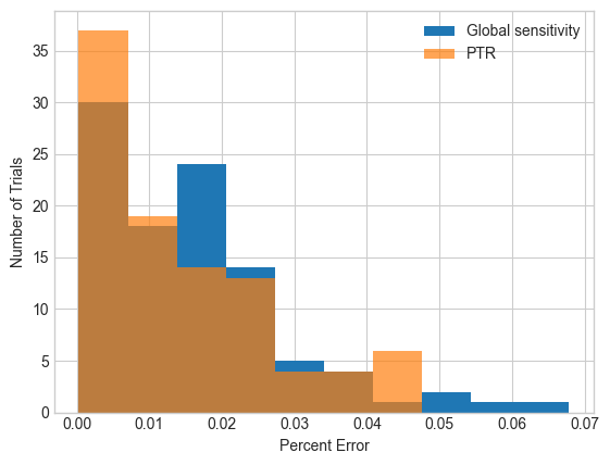
We might do slightly better with propose-test-release, but it’s not a huge difference. Moreover, to use propose-test-release, the analyst has to propose a bound on sensitivity - and we’ve cheated by “magically” picking a decent value (0.005). In practice, the analyst would need to perform several queries to explore which values work - which will consume additional privacy budget.

Smooth Sensitivity#

Our second approach for leveraging local sensitivity is called smooth sensitivity [18]. The smooth sensitivity framework, instantiated with Laplace noise, provides \((\epsilon, \delta)\)-differential privacy:

Definition 19 (Smooth Sensitivity Framework)

Set \(\beta = \frac{\epsilon}{2\log(2/\delta)}\)
Let \(S = \max_{k = 1, \dots, n} e^{-\beta k} A(f, x, k)\)
Release \(f(x) + \mathsf{Lap}\left(\frac{2S}{\epsilon}\right)\)

The idea behind smooth sensitivity is to use a “smooth” approximation of local sensitivity, rather than local sensitivity itself, to calibrate the noise. The amount of smoothing is designed to prevent the unintentional release of information about the dataset that can happen when local sensitivity is used directly. Step 2 above performs the smoothing: it scales the local sensitivity of nearby datasets by an exponential function of their distance from the actual dataset, then takes the maximum scaled local sensitivity. The effect is that if a spike in local sensitivity exists in the neighborhood of \(x\), that spike will be reflected in the smooth sensitivity of \(x\) (and therefore the spike itself is “smoothed out,” and doesn’t reveal anything about the dataset).

Smooth sensitivity has a significant advantage over propose-test-release: it doesn’t require the analyst to propose a bound on sensitivity. For the analyst, using smooth sensitivity is just as easy as using global sensitivity. However, smooth sensitivity has two major drawbacks. First, smooth sensitivity is always larger than local sensitivity (by at least a factor of 2 - see step 3), so it may require adding quite a bit more noise than alternative frameworks like propose-test-release (or even global sensitivity). Second, calculating smooth sensitivity requires finding the maximum smoothed-out sensitivity over all possible values for \(k\), which can be extremely challenging computationally. In many cases, it’s possible to prove that considering a small number of values for \(k\) is sufficient (for many functions, the exponentially decaying \(e^{-\beta k}\) quickly overwhelms the growing value of \(A(f, x, k)\)), but such a property has to be proven for each function we want to use with smooth sensitivity.

As an example, let’s consider the smooth sensitivity of the mean query we defined earlier.

Final sensitivity: 0.006141751627564181

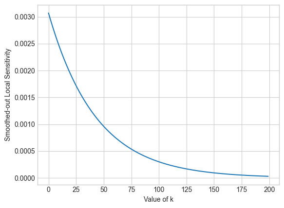
_images/a179fbffd18dadf7e4d57e8ffd767d691d91eef04a5320af602e907584005185.png

There are two things to notice here. First, even though we consider only values of \(k\) less than 200, it’s pretty clear that the smoothed-out local sensitivity of our mean query approaches 0 as \(k\) grows. In fact, for this case, the maximum occurs at \(k=0\). This is true in many cases, but if we want to use smooth sensitivity, we have to prove it (which we won’t do here). Second, notice that the final sensitivity we’ll use for adding noise to the query’s answer is higher than the sensitivity we proposed earlier (under propose-test-release). It’s not a big difference, but it shows that it’s sometimes possible to achieve a lower sensitivity with propose-test-release than with smooth sensitivity.

Sample and Aggregate#

We’ll consider one last framework related to local sensitivity, called sample and aggregate [18]. For any function \(f : D \rightarrow \mathbb{R}\) and upper and lower clipping bounds \(u\) and \(l\), the following framework satisfies \(\epsilon\)-differential privacy:

Definition 20 (Sample And Aggregate Framework)

Split the dataset \(X \in D\) into \(k\) disjoint chunks \(x_1, \dots, x_k\)
Compute a clipped answer for each chunk: \(a_i = \max(l, \min(u, f(x_i)))\)
Compute a noisy average of the answers: \(A = \left(\frac{1}{k} \sum_{i=1}^k a_i \right) + \mathsf{Lap}\left(\frac{u - l}{k\epsilon}\right)\)

Note that this framework satisfies pure \(\epsilon\)-differential privacy, and it actually works without the use of local sensitivity. In fact, we don’t need to know anything about the sensitivity of \(f\) (global or local). We also don’t need to know anything about the chunks \(x_i\), except that they’re disjoint. Often, they’re chosen randomly (“good” samples tend to result in higher accuracy), but they don’t need to be.

The framework can be shown to satisfy differential privacy just by global sensitivity and parallel composition. We split the dataset into \(k\) distinct chunks, so each individual appears in exactly one chunk. We don’t know the sensitivity of \(f\), but we clip its output to lie between \(u\) and \(l\), so the sensitivity of each clipped answer \(f(x_i)\) is \(u-l\). Since we take the mean of \(k\) invocations of \(f\), the global sensitivity of the mean is \(\frac{u-l}{k}\).

Note that we’re claiming a bound on the global sensitivity of a mean directly, rather than splitting it into sum and count queries. We weren’t able to do this for “regular” mean queries, because the number of things being averaged in a “regular” mean query depends on the dataset. In this case, however, the number of items being averaged is fixed by the analyst, via the choice of \(k\) - it’s independent of the dataset. Mean queries like this one - where the number of things being averaged is fixed, and can be made public - can leverage this improved bound on global sensitivity.

In this simple instantiation of the sample and aggregate framework, we ask the analyst to provide the upper and lower bounds \(u\) and \(l\) on the output of each \(f(x_i)\). Depending on the definition of \(f\), this might be extremely difficult to do well. In a counting query, for example, \(f\)’s output will depend directly on the dataset.

More advanced instantiations have been proposed which leverage local sensitivity to avoid asking the analyst for \(u\) and \(l\). For some functions, however, bounding \(f\)’s output is easy - so this framework suffices. We’ll consider our example from above - the mean of ages within a dataset - with this property. The mean age of a population is highly likely to fall between 20 and 80, so it’s reasonable to set \(l=20\) and \(u=80\). As long as our chunks \(x_i\) are each representative of the population, we’re not likely to lose much information with this setting.

The key parameter in this framework is the number of chunks, \(k\). As \(k\) goes up, the sensitivity of the final noisy mean goes down - so more chunks means less noise. On the other hand, as \(k\) goes up, each chunk gets smaller, so each answer \(f(x_i)\) is less likely to be close to the “true” answer \(f(X)\). In our example above, we’d like the average age within each chunk to be close to the average age of the whole dataset - and this is less likely to happen if each chunk contains only a handful of people.

How should we set \(k\)? It depends on \(f\) and on the dataset, which makes it tricky. Let’s try various values of \(k\) for our mean query over the \(Age\) feature.

def plot_results(k):
    df = adult['Age']
    true_avg = np.mean(df)

    # First histogram: Sample-and-Aggregate (SAA) mechanism
    saa_errors = [pct_error(true_avg, saa_avg_age(k, epsilon)) for _ in range(100)]
    _, bins, _ = plt.hist(saa_errors, label='Sample-and-Aggregate (SAA)', alpha=0.7)

    # Second histogram: Global Sensitivity (GS) mechanism
    gs_errors = [pct_error(true_avg, gs_avg(df, u, epsilon)) for _ in range(100)]
    plt.hist(gs_errors, alpha=0.7, bins=bins, label='Global Sensitivity (GS)')

    # Add title and legend
    plt.title(f'Percent Error in Average Age (k={k})')
    plt.xlabel('Percent Error')
    plt.ylabel('Frequency')
    plt.legend()
    plt.grid(True)
    plt.tight_layout()

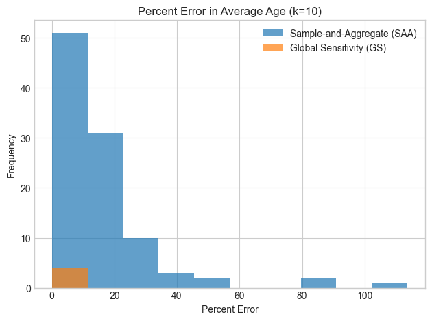
# k = 10; global sensitivity is *much* better
plot_results(10)

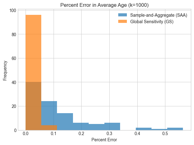
_images/16ff63bcc900facc9e6740f7a4f1e36e7e75983c8f16748ecfc215aec5f5852c.png

# k = 1000; global sensitivity is still better
plot_results(1000)

_images/a1b6626381658d74957faea41d58ed5e651837a08a1fb57e1a0a1f5a25e26c7d.png

# k = 6000; sample and aggregate is getting close!
plot_results(6000)

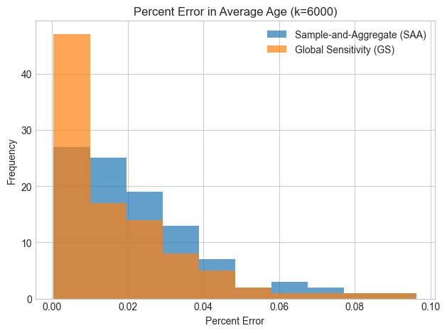
_images/6ef1cff56614e9da0cba23192c50e986392e09136c690ce904fc8acac7ea4318.png

So - sample and aggregate isn’t able to beat our global sensitivity-based approach, but it can get pretty close if you choose the right value for \(k\). The big advantage is that sample and aggregate works for any function \(f\), regardless of its sensitivity; if \(f\) is well-behaved, then it’s possible to obtain good accuracy from the framework. On the other hand, using sample and aggregate requires the analyst to set the clipping bounds \(u\) and \(l\), and the number of chunks \(k\).

Note

Choosing Between PTR, Smooth Sensitivity, and Sample-and-Aggregate

Several advanced techniques exist for releasing statistics under differential privacy when global sensitivity is too high or poorly behaved. These include Propose-Test-Release, Smooth Sensitivity, and Sample-and-Aggregate. Each method provides a way to adapt to local characteristics of the data, but they differ in applicability, complexity, and robustness. This section offers practical guidance on when to use each.

Propose-Test-Release (PTR)

Use PTR when:

You are working with a bounded, well-behaved statistic, like a median or mode.
You expect the statistic to be stable on the dataset (i.e., unlikely to change much if a single row is added or removed).
You can define a testable notion of stability, such as a small local sensitivity.
It’s acceptable to occasionally suppress output if the stability test fails.

PTR is conceptually simple and efficient, but it may fail to release an output on unstable datasets. This makes it ideal for use cases like releasing a median salary from a large population, but less suitable in adversarial or highly variable data settings.

Smooth Sensitivity

Use Smooth Sensitivity when:

You need to release a scalar statistic, like the median or interquartile range.
The local sensitivity varies widely, and a tighter bound is needed than global sensitivity.
You want graceful degradation: when the data is stable, you get low noise; when it’s unstable, you still get a private result (with higher noise).
You can compute or bound the smooth sensitivity efficiently (e.g., with closed-form expressions or approximations).

Smooth sensitivity is powerful but can be mathematically and computationally involved, especially when estimating the maximum local sensitivity over nearby datasets. It is preferred when accuracy is critical and the statistic is inherently unstable (e.g., publishing the median of a skewed dataset).

Sample-and-Aggregate (SAA)

Use SAA when:

You want to release an arbitrary statistic, including complex or non-numeric outputs (e.g., model parameters, clustering results).
The statistic is not globally stable, but becomes stable when computed on smaller subsamples.
You are able to partition the dataset into sufficiently many disjoint chunks of similar size.
You can define a private aggregator, such as the noisy median or mode of subsample outputs.

SAA offers broad flexibility, but its accuracy depends on the number and size of partitions. It is particularly useful when applying non-differentially private procedures (like training a model) privately by aggregating across partitions. However, the method may degrade when sample sizes are small or outputs are highly variable across groups.

Method	Use When…	Caution
PTR	Statistic is stable and you can test it	May suppress output on unstable data
Smooth Sensitivity	Need high accuracy for scalar statistics	Harder to compute; less scalable
Sample-and-Aggregate	Statistic is complex or arbitrary	Depends on effective partitioning and noise

Each of these tools allows you to work beyond global sensitivity, which is often too conservative. Choosing the right method depends on the data distribution, your tolerance for failure or noise, and the type of statistic you’re trying to release.

Glossary