Sensitivity#
Learning Objectives
After reading this chapter, you will be able to:
Define sensitivity
Find the sensitivity of counting queries
Find the sensitivity of summation queries
Decompose average queries into counting and summation queries
Use clipping to bound the sensitivity of summation queries
As we mentioned when we discussed the Laplace mechanism, the amount of noise necessary to ensure differential privacy for a given query depends on the sensitivity of the query. Roughly speaking, the sensitivity of a function reflects the amount the function’s output will change when its input changes. Recall that the Laplace mechanism defines a mechanism \(F(x)\) as follows:
where \(f(x)\) is a deterministic function (the query), \(\epsilon\) is the privacy parameter, and \(s\) is the sensitivity of \(f\).
For a function \(f : \mathcal{D} \rightarrow \mathbb{R}\) mapping datasets (\(\mathcal{D}\)) to real numbers, the global sensitivity of \(f\) is defined as follows:
Definition 7 (Global Sensitivity)
Here, \(d(x, x')\) represents the distance between two datasets \(x\) and \(x'\), and we say that two datasets are neighbors if their distance is 1 or less. How this distance is defined has a huge effect on the definition of privacy we obtain, and we’ll discuss the distance metric on datasets in detail later on.
The definition of global sensitivity says that for any two neighboring datasets \(x\) and \(x'\), the difference between \(f(x)\) and \(f(x')\) is at most \(GS(f)\). This measure of sensitivity is called “global” because it is independent of the actual dataset being queried (it holds for any choice of neighboring \(x\) and \(x'\)). Another measure of sensitivity, called local sensitivity, fixes one of the datasets to be the one being queried; we will consider this measure in a later section. For now, when we say “sensitivity,” we mean global sensitivity.
Distance#
The distance metric \(d(x,x')\) described earlier can be defined in many different ways. Intuitively, the distance between two datasets should be equal to 1 (i.e. the datasets are neighbors) if they differ in the data of exactly one individual. This idea is easy to formalize in some contexts (e.g. in the US Census, each individual submits a single response containing their data) but extremely challenging in others (e.g. location trajectories, social networks, and time-series data).
A common formal definition for datasets containing rows is to consider the number of rows which differ between the two. When each individual’s data is contained in a single row, this definition often makes sense. Formally, this definition of distance is encoded as a symmetric difference between the two datasets:
Definition 8 (Symmetric Difference)
This particular definition has several interesting and important implications:
If \(x'\) is constructed from \(x\) by adding one row, then \(d(x,x') = 1\)
If \(x'\) is constructed from \(x\) by removing one row, then \(d(x,x') = 1\)
If \(x'\) is constructed from \(x\) by modifying one row, then \(d(x,x') = 2\)
In other words, adding or removing a row results in a neighboring dataset; modifying a row results in a dataset at distance 2.
This particular definition of distance results in what is typically called unbounded differential privacy. Many other definitions are possible, including one called bounded differential privacy in which modifying a single row in a dataset does result in a neighboring dataset.
For now, we will stick to the formal definition defined above in terms of symmetric difference. We will discuss alternative definitions in a later section.
Calculating Sensitivity#
How do we determine the sensitivity of a particular function of interest? For some simple functions on real numbers, the answer is obvious.
The global sensitivity of \(f(x) = x\) is 1, since changing \(x\) by 1 changes \(f(x)\) by 1
The global sensitivity of \(f(x) = x+x\) is 2, since changing \(x\) by 1 changes \(f(x)\) by 2
The global sensitivity of \(f(x) = 5*x\) is 5, since changing \(x\) by 1 changes \(f(x)\) by 5
The global sensitivity of \(f(x) = x*x\) is unbounded, since the change in \(f(x)\) depends on the value of \(x\)
For functions that map datasets to real numbers, we can perform a similar analysis. We will consider the functions which represent common aggregate database queries: counts, sums, and averages.
Counting Queries#
Counting queries (COUNT in SQL) count the number of rows in the dataset which satisfy a specific property. As a rule of thumb, counting queries always have a sensitivity of 1. This is because adding a row to the dataset can increase the output of the query by at most 1: either the new row has the desired property, and the count increases by 1, or it does not, and the count stays the same (the count may correspondingly decrease when a row is removed).
Example: “How many people are in the dataset?” (sensitivity: 1 - counting rows where the property = True)
adult.shape[0]
32563
Example: “How many people have an educational status above 10?” (sensitivity: 1 - counting rows with a property)
adult[adult['Education-Num'] > 10].shape[0]
10517
Example: “How many people have an educational status equal to or below 10?” (sensitivity: 1 - counting rows with a property)
adult[adult['Education-Num'] <= 10].shape[0]
22046
Example: “How many people are named Joe Near?” (sensitivity: 1 - counting rows with a property)
adult[adult['Name'] == 'Joe Near'].shape[0]
0
Summation Queries#
Summation queries (SUM in SQL) sum up the attribute values of dataset rows.
Example: “What is the sum of the ages of people with an educational status above 10?”
adult[adult['Education-Num'] > 10]['Age'].sum()
441431
Sensitivity for these queries is not as simple as it is for counting queries. Adding a new row to the dataset will increase the result of our example query by the age of the new person. That means the sensitivity of the query depends on the contents of the row we add.
We’d like to come up with a concrete number to represent the sensitivity of the query. Unfortunately, no number really exists. We could claim, for example, that the sensitivity is 125 - but it may turn out that the row we add to the database corresponds to a person who is over 125 years old, which would violate our claim. For any number we come up with, it’s possible for the added row to violate our claim.
You might (rightly) be skeptical of this point. Say we claim the sensitivity is 1000 - it’s very unlikely that we’ll find a person who is 1000 years old to violate this claim. In this specific domain - ages - there’s a very reasonable upper bound on how old someone can be. The oldest person ever lived to be 122 years old, so an upper bound of 125 seems reasonable.
But this is not a proof that nobody will ever live to be 126. And in other domains (e.g. income), it can be much harder to come up with a reasonable upper bound.
As a rule of thumb, summation queries have unbounded sensitivity when no lower and upper bounds exist on the value of the attribute being summed. When lower and upper bounds do exist, the sensitivity of a summation query is equal to the difference between them. In the next section, we will see a technique called clipping for enforcing bounds when none exist, so that summation queries with unbounded sensitivity can be converted into queries with bounded sensitivity.
Average Queries#
Average queries (AVG in SQL) calculate the mean of attribute values in a particular column.
Example: “What is the average age of people with an educational status above 10?”
adult[adult['Education-Num'] > 10]['Age'].mean()
41.973091185699346
The easiest way to answer an average query with differential privacy is by re-phrasing it as two queries: a summation query divided by a counting query. For the above example:
adult[adult['Education-Num'] > 10]['Age'].sum() / adult[adult['Education-Num'] > 10]['Age'].shape[0]
41.973091185699346
The sensitivities of both queries can be calculated as described above. Noisy answers for each can be calculated (e.g. using the Laplace mechanism) and the noisy answers can be divided to obtain a differentially private mean. The total privacy cost of both queries can be calculated by sequential composition.
Clipping#
Queries with unbounded sensitivity cannot be directly answered with differential privacy using the Laplace mechanism. Fortunately, we can often transform such queries into equivalent queries with bounded sensitivity, via a process called clipping.
The basic idea behind clipping is to enforce upper and lower bounds on attribute values. For example, ages above 125 can be “clipped” to exactly 125. After clipping has been performed, we are guaranteed that all ages will be 125 or below. As a result, the sensitivity of a summation query on clipped data is equal to the difference between the upper and lower bounds used in clipping: \(upper - lower\). For example, the following query has a sensitivity of 125:
adult['Age'].clip(lower=0, upper=125).sum()
1360238
The primary challenge in performing clipping is to determine the upper and lower bounds. For ages, this is simple - nobody can have an age less than 0, and probably nobody will be older than 125. In other domains, as mentioned earlier, it’s much more difficult.
Furthermore, there is a tradeoff between the amount of information lost in clipping and the amount of noise needed to ensure differential privacy. When the upper and lower clipping bounds are closer together, then the sensitivity is lower, and less noise is needed to ensure differential privacy. However, aggressive clipping often removes a lot of information from the data; this information loss tends to cause a loss of accuracy which outweighs the improvement in noise resulting from smaller sensitivity.
As a rule of thumb, try to set the clipping bounds to include 100% of the dataset, or get as close as possible. This is harder in some domains (e.g. graph queries, which we will study later) than others.
It’s tempting to determine the clipping bounds by looking at the data. For example, we can look at the histogram of ages in our dataset to determine an appropriate upper bound:
Show code cell source
plt.hist(adult['Age'])
plt.xlabel('Age')
plt.ylabel('Number of Records');
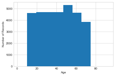
It’s clear from this histogram that nobody in this particular dataset is over 90, so an upper bound of 90 would suffice.
However, it’s important to note that this approach does not satisfy differential privacy. If we pick our clipping bounds by looking at the data, then the bounds themselves might reveal something about the data.
Typically, clipping bounds are decided either by using a property of the dataset that can be known without looking at the data (e.g. that the dataset contains ages, which are likely to lie between 0 and 125), or by performing differentially private queries to evaluate different choices for the clipping bounds.
To use the second approach, we typically set the lower bound to 0 and slowly increase the upper bound until the query’s output stops changing (meaning we haven’t included any new data by increasing the bound). For example, let’s try computing the sum of ages for clipping bounds from 0 to 100, using the Laplace mechanism for each one to ensure differential privacy:
Show code cell source
def laplace_mech(v, sensitivity, epsilon):
    return v + np.random.laplace(loc=0, scale=sensitivity/epsilon)

epsilon_i = .01
plt.plot([laplace_mech(adult['Age'].clip(lower=0, upper=i).sum(), i, epsilon_i) for i in range(100)])
plt.xlabel('Clipping Bound for Age')
plt.ylabel('Total Sum');
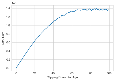
The total privacy cost for building this plot is \(\epsilon = 1\) by sequential composition, since we do 100 queries each with \(\epsilon_i = 0.01\). It’s clear that the results level off around a value of upper = 80, so this is a good choice for the clipping bound.
We can use the same approach for data attributes from any numerical domain, but it helps to know something about the scale of the data in advance. For example, trying clipping values between 0 and 100 for yearly incomes would not work very well - we wouldn’t even come close to finding a reasonable upper bound.
One refinement that can work well when the scale of the data is not known is to test upper bounds according to a logarithmic scale.
Show code cell source
xs = [2**i for i in range(15)]
plt.plot(xs, [laplace_mech(adult['Age'].clip(lower=0, upper=i).sum(), i, epsilon_i) for i in xs])
plt.xscale('log')
plt.xlabel('Clipping Bound for Age')
plt.ylabel('Total Sum');
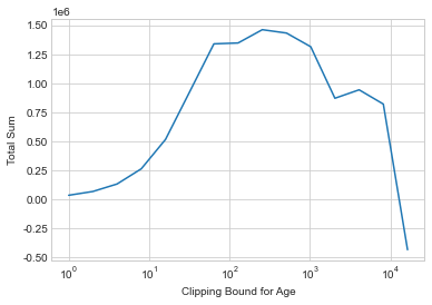
This approach allows us to test a huge range of possible bounds with a small number of queries, but at the expense of less precision in determining the perfect bound. As the upper bound gets really large, the noise will start to overwhelm the signal - notice how the sum fluctuates wildly for the largest clipping parameters! The key is to look for a region of the graph which is relatively smooth (meaning low noise) and also not increasing (meaning the clipping bound is sufficient). Here, this occurs at roughly \(2^8 = 256\), which is a reasonable approximation of the upper bound we derived earlier.
Avoiding Sensitivity Underestimation#
In order to correctly predict the sensitivity of our queries and tranformations, we rely on mathematical reasoning around numeric functions such as arithmetic operators.
If for some reason our numeric functions failed to properly work as anticipated, this would throw off our sensitivity analysis. This could happen, for example, when integer overflow or floating-point representation error occur [14, 15].
0.1 + 0.2
0.30000000000000004
Oh no! In this example, due to representation error of floating-point numbers in Python, our result is slightly larger than expected.
This means that there is the potential of sensitivity underestimation in any numeric operations which naively add floating-point number types in Python.
Fortunately, there are several ways to remedy this issue - in Python and other programming languages - for example via truncation and rounding, for which there are several techniques. In many cases these techniques dance around trading efficiency for increased precision.
For example, in Python we can achieve arbitrary precision via the decimal module which provides support for fast correctly rounded decimal floating-point arithmetic.
from decimal import *

Decimal('0.1') + Decimal('0.2')
Decimal('0.3')
Using this approach, we achieve the correct result, and the correctness of our sensitivity analysis is preserved.
This is made possible through use of the Python Decimal module.
Tip
In Python3 integers have arbitrary size which is only limited by available memory. This means that we don’t normally need to worry about integer overflow affecting the correctness of our sensitivity analysis.
Sensitivity underestimation may break the differential privacy guarantee, while sensitivity overestimation leads to unnecessary inaccuracy in the private analysis.
Summary
The amount of noise necessary to ensure differential privacy for a given query depends on the sensitivity of the query.
Roughly speaking, the sensitivity of a function reflects the amount the function’s output will change when its input changes.
Intuitively, the distance between two datasets should be equal to 1 (i.e. the datasets are neighbors) if they differ in the data of exactly one individual.
Queries with unbounded sensitivity cannot be directly answered with differential privacy using the Laplace mechanism.
Fortunately, we can often transform such queries into equivalent queries with bounded sensitivity, via a process called clipping.
In order to correctly predict the sensitivity of our queries and tranformations, we rely on mathematical reasoning around numeric functions.
Sensitivity underestimation may break the differential privacy guarantee, while sensitivity overestimation leads to unnecessary inaccuracy in the private analysis.
Glossary
numpy.clip(): Clip values to a specified min and max.numpy.abs(): Compute absolute values.numpy.linalg.norm(): Compute vector norms.